In general, there is no closed form solution to these integrals, and we have to approximate them numerically. The first step is to check if there is some reparameterization that will simplify the problem. Then, the general approaches to solving integration problems are
This lecture will review the concepts for quadrature and Monte Carlo integration.
You may recall from Calculus that integrals can be numerically evaluated using quadrature methods such as Trapezoid and Simpson’s‘s rules. This is easy to do in Python, but has the drawback of the complexity growing as \(O(n^d)\) where \(d\) is the dimensionality of the data, and hence infeasible once \(d\) grows beyond a modest number.
from scipy.integrate import quad
def f(x): return x * np.cos(71*x) + np.sin(13*x)
x = np.linspace(0, 1, 100) plt.plot(x, f(x)) pass
from sympy import sin, cos, symbols, integrate x = symbols('x') integrate(x * cos(71*x) + sin(13*x), (x, 0,1)).evalf(6)
0.0202549
y, err = quad(f, 0, 1.0) y
0.02025493910239419
Following the scipy.integrate documentation, we integrate
\[I=\int_x, y = symbols('x y') integrate(x*y, (x, 0, 1-2*y), (y, 0, 0.5))
0.0104166666666667
from scipy.integrate import nquad def f(x, y): return x*y def bounds_y(): return [0, 0.5] def bounds_x(y): return [0, 1-2*y] y, err = nquad(f, [bounds_x, bounds_y]) y
0.010416666666666668
The basic idea of Monte Carlo integration is very simple and only requires elementary statistics. Suppose we want to find the value of
\[I = \int_a^b f(x) dx\]in some region with volume \(V\) . Monte Carlo integration estimates this integral by estimating the fraction of random points that fall below \(f(x)\) multiplied by \(V\) .
In a statistical context, we use Monte Carlo integration to estimate the expectation
\[E[g(X)] = \int_X g(x) p(x) dx\] \[\barwhere \(x_i \sim p\) is a draw from the density \(p\) .
We can estimate the Monte Carlo variance of the approximation as
\[v_n = \frac<1> \sum_^n (g(x_i) - \bar)^2)\]Also, from the Central Limit Theorem,
\[\frac - E[g(X)]>> \sim \mathcal(0, 1)\]The convergence of Monte Carlo integration is \(\mathcal(n^)\) and independent of the dimensionality. Hence Monte Carlo integration generally beats numerical integration for moderate- and high-dimensional integration since numerical integration (quadrature) converges as \(\mathcal(n^)\) . Even for low dimensional problems, Monte Carlo integration may have an advantage when the volume to be integrated is concentrated in a very small region and we can use information from the distribution to draw samples more often in the region of importance.An elementary, readable description of Monte Carlo integration and variance reduction techniques can be found here.
We want to find some integral
\[I = \int \, dx\]Consider the expectation of a function \(g(x)\) with respect to some distribution \(p(x)\) . By definition, we have
If we choose \(g(x) = f(x)/p(x)\) , then we have
\[\beginBy the law of large numbers, the average converges on the expectation, so we have
\[I \approx \barIf \(f(x)\) is a proper integral (i.e. bounded), and \(p(x)\) is the uniform distribution, then \(g(x) = f(x)\) and this is known as ordinary Monte Carlo. If the integral of \(f(x)\) is improper, then we need to use another distribution with the same support as \(f(x)\) .
We will just work this out for a proper integral \(f(x)\) defined in the unit cube and bounded by \(|f(x)| \le 1\) . Draw a random uniform vector \(x\) in the unit cube. Then
Now consider summing over many such IID draws \(S_n = f(x_1) + f(x_2) + \cdots + f(x_n)\) . We have
\[\beginand as expected, we see that \(I \approx S_n/n\) . From Chebyshev’s inequality,
\[\begin
Suppose we want 1% accuracy and 99% confidence - i.e. set \(\epsilon = \delta = 0.01\) . The above inequality tells us that we can achieve this with just \(n = 1/(\delta \epsilon^2) = 1,000,000\) samples, regardless of the data dimensionality.
We want to estimate the following integral \(\int_0^1 e^x dx\) . The minimum value of the function is 1 at \(x=0\) and \(e\) at \(x=1\) .
x = np.linspace(0, 1, 100) plt.plot(x, np.exp(x)) plt.xlim([0,1]) plt.ylim([0, np.e]) pass

from sympy import symbols, integrate, exp x = symbols('x') expr = integrate(exp(x), (x,0,1)) expr.evalf()
1.71828182845905
from scipy import integrate y, err = integrate.quad(exp, 0, 1) y
1.7182818284590453
for n in 10**np.array([1,2,3,4,5,6,7,8]): x = np.random.uniform(0, 1, n) sol = np.mean(np.exp(x)) print('%10d %.6f' % (n, sol))
10 1.657995 100 1.736252 1000 1.712426 10000 1.718823 100000 1.718524 1000000 1.718875 10000000 1.718498 100000000 1.718227
We are often interested in knowing how many iterations it takes for Monte Carlo integration to “converge”. To do this, we would like some estimate of the variance, and it is useful to inspect such plots. One simple way to get confidence intervals for the plot of Monte Carlo estimate against number of iterations is simply to do many such simulations.
For the example, we will try to estimate the function (again)
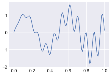
\[f(x) = x \cos 71 x + \sin 13x, \ \ 0 \le x \le 1\]def f(x): return x * np.cos(71*x) + np.sin(13*x)
x = np.linspace(0, 1, 100) plt.plot(x, f(x)) pass

n = 100 x = f(np.random.random(n)) y = 1.0/n * np.sum(x) y
-0.13559989390095498
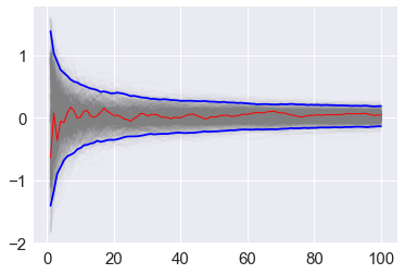
We vary the sample size from 1 to 100 and calculate the value of \(y = \sum/n\) for 1000 replicates. We then plot the 2.5th and 97.5th percentile of the 1000 values of \(y\) to see how the variation in \(y\) changes with sample size. The blue lines indicate the 2.5th and 97.5th percentiles, and the red line a sample path.
n = 100 reps = 1000 x = f(np.random.random((n, reps))) y = 1/np.arange(1, n+1)[:, None] * np.cumsum(x, axis=0) upper, lower = np.percentile(y, [2.5, 97.5], axis=1)
plt.plot(np.arange(1, n+1), y, c='grey', alpha=0.02) plt.plot(np.arange(1, n+1), y[:, 0], c='red', linewidth=1); plt.plot(np.arange(1, n+1), upper, 'b', np.arange(1, n+1), lower, 'b') pass
If it is too expensive to do 1000 replicates, we can use a bootstrap instead.
xb = np.random.choice(x[:,0], (n, reps), replace=True) yb = 1/np.arange(1, n+1)[:, None] * np.cumsum(xb, axis=0) upper, lower = np.percentile(yb, [2.5, 97.5], axis=1)
plt.plot(np.arange(1, n+1)[:, None], yb, c='grey', alpha=0.02) plt.plot(np.arange(1, n+1), yb[:, 0], c='red', linewidth=1) plt.plot(np.arange(1, n+1), upper, 'b', np.arange(1, n+1), lower, 'b') pass

With independent samples, the variance of the Monte Carlo estimate is
where \(Y_i = f(x_i)/p(x_i)\) . The objective of Monte Carlo swindles is to make \(\text[\bar]\) as small as possible for the same number of samples.
The Cauchy distribution is given by
\[f(x) = \frac<1><\pi (1 + x^2)>, \ \ -\infty \lt x \lt \infty\]Suppose we want to integrate the tail probability \(P(X > 3)\) using Monte Carlo. One way to do this is to draw many samples form a Cauchy distribution, and count how many of them are greater than 3, but this is extremely inefficient.
import scipy.stats as stats h_true = 1 - stats.cauchy().cdf(3) h_true
0.10241638234956674
n = 100 x = stats.cauchy().rvs(n) h_mc = 1.0/n * np.sum(x > 3) h_mc, np.abs(h_mc - h_true)/h_true
(0.14000000000000001, 0.36696880702301304)
We are trying to estimate the quantity
\[\int_3^\infty \frac<1> <\pi (1 + x^2)>dx\]Using the substitution \(y = 3/x\) (and a little algebra), we get
\[\int_0^1 \frac<3> <\pi(9 + y^2)>dy\]Hence, a much more efficient MC estimator is
\[\frac<1> \sum_^n \frac<\pi(9 + y_i^2)>\]where \(y_i \sim \mathcal(0, 1)\) .
y = stats.uniform().rvs(n) h_cv = 1.0/n * np.sum(3.0/(np.pi * (9 + y**2))) h_cv, np.abs(h_cv - h_true)/h_true
(0.10213456867129996, 0.0027516464827364996)
Apart from change of variables, there are several general techniques for variance reduction, sometimes known as Monte Carlo swindles since these methods improve the accuracy and convergence rate of Monte Carlo integration without increasing the number of Monte Carlo samples. Some Monte Carlo swindles are:
Most of these techniques are not particularly computational in nature, so we will not cover them in the course. I expect you will learn them elsewhere. We will illustrate importance sampling and antithetic variables here as examples.
The idea behind antithetic variables is to choose two sets of random numbers that are negatively correlated, then take their average, so that the total variance of the estimator is smaller than it would be with two sets of IID random variables.
def f(x): return x * np.cos(71*x) + np.sin(13*x)
from sympy import sin, cos, symbols, integrate x = symbols('x') sol = integrate(x * cos(71*x) + sin(13*x), (x, 0,1)).evalf(16) sol
0.02025493910239406
n = 10000 u = np.random.random(n) x = f(u) y = 1.0/n * np.sum(x) y, abs(y-sol)/sol
(0.019429826681871879, 0.04073635651783584)
This works because the random draws are now negatively correlated, and hence the sum of the variances will be less than in the IID case, while the expectation is unchanged.
u = np.r_[u[:n//2], 1-u[:n//2]] x = f(u) y = 1.0/n * np.sum(x) y, abs(y-sol)/sol
(0.021069877090343692, 0.04023403792180801)
Ordinary Monte Carlo sampling evaluates
\[E[g(X)] = \int_X g(x)\, p(x) \, dx\]Using another distribution \(h(x)\) - the so-called “importance function”, we can rewrite the above expression as an expectation with respect to \(h\)
\[E_p[g(x)] \ = \ \int_X g(x) \frac h(x) dx \ = \ E_h\left[ \frac \right]\]giving us the new estimator
\[\barwhere \(x_i \sim g\) is a draw from the density \(h\) . This is helpful if the distribution \(h\) has a similar shape as the function \(f(x)\) that we are integrating over, since we will draw more samples from places where the integrand makes a larger or more “important” contribution. This is very dependent on a good choice for the importance function \(h\) . Two simple choices for \(h\) are scaling
In these cases, the parameter \(a\) is typically chosen using some adaptive algorithm, giving rise to adaptive importance sampling. Alternatively, a different distribution can be chosen as shown in the example below.
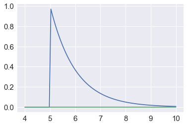
Suppose we want to estimate the tail probability of \(\mathcal(0, 1)\) for \(P(X > 5)\) . Regular MC integration using samples from \(\mathcal(0, 1)\) is hopeless since nearly all samples will be rejected. However, we can use the exponential density truncated at 5 as the importance function and use importance sampling.
x = np.linspace(4, 10, 100) plt.plot(x, stats.expon(5).pdf(x)) plt.plot(x, stats.norm().pdf(x)) pass
We expect about 3 draws out of 10,000,000 from \(\mathcal(0, 1)\) to have a value greater than 5. Hence simply sampling from \(\mathcal(0, 1)\) is hopelessly inefficient for Monte Carlo integration.
%precision 10
h_true =1 - stats.norm().cdf(5) h_true
0.0000002867
n = 10000 y = stats.norm().rvs(n) h_mc = 1.0/n * np.sum(y > 5) # estimate and relative error h_mc, np.abs(h_mc - h_true)/h_true
(0.0000000000, 1.0000000000)
n = 10000 y = stats.expon(loc=5).rvs(n) h_is = 1.0/n * np.sum(stats.norm().pdf(y)/stats.expon(loc=5).pdf(y)) # estimate and relative error h_is, np.abs(h_is- h_true)/h_true
(0.0000002944, 0.0270524683)
Recall that the convergence of Monte Carlo integration is \(\mathcal(n^)\) . One issue with simple Monte Carlo is that randomly chosen points tend to be clumped. Clumping reduces accuracy since nearby points provide little additional information about the function begin estimated. One way to address this is to split the space into multiple integration regions, then sum them up. This is known as stratified sampling. Another alternative is to use quasi-random numbers which fill space more efficiently than random sequences
It turns out that if we use quasi-random or low discrepancy sequences, we can get convergence approaching \(\mathcal(1/n)\) . There are several such generators, but their use in statistical settings is limited to cases where we are integrating with respect to uniform distributions. The regularity can also give rise to errors when estimating integrals of periodic functions. However, these quasi-Monte Carlo methods are used in computational finance models.
! pip install ghalton
if ghalton is not installed.
import ghalton gen = ghalton.Halton(2)
plt.figure(figsize=(10,5)) plt.subplot(121) xs = np.random.random((100,2)) plt.scatter(xs[:, 0], xs[:,1]) plt.axis([-0.05, 1.05, -0.05, 1.05]) plt.title('Pseudo-random', fontsize=20) plt.subplot(122) ys = np.array(gen.get(100)) plt.scatter(ys[:, 0], ys[:,1]) plt.axis([-0.05, 1.05, -0.05, 1.05]) plt.title('Quasi-random', fontsize=20);

h_true = 1 - stats.cauchy().cdf(3)
n = 10 x = stats.uniform().rvs((n, 5)) y = 3.0/(np.pi * (9 + x**2)) h_mc = np.sum(y, 0)/n list(zip(h_mc, 100*np.abs(h_mc - h_true)/h_true))
[(0.0995639331, 2.7851493922), (0.1013519751, 1.0392939477), (0.1018614640, 0.5418257479), (0.1006039674, 1.7696533966), (0.1030816150, 0.6495373689)]
gen1 = ghalton.Halton(1) x = np.reshape(gen1.get(n*5), (n, 5)) y = 3.0/(np.pi * (9 + x**2)) h_qmc = np.sum(y, 0)/n list(zip(h_qmc, 100*np.abs(h_qmc - h_true)/h_true))
[(0.1026632536, 0.2410466633), (0.1023042949, 0.1094428682), (0.1026741252, 0.2516617574), (0.1029118212, 0.4837496311), (0.1026111501, 0.1901724534)]